Lambda Power Tuning Case Study 🔧

Intro

There are two metrics for costing an AWS Lambda invocation, the memory size and running duration. Since we’re charged by GB-seconds in Lambda, the faster our lambda executes, the less we’ll be charged. Because of this, we could increase memory (and therefore more vCPU), yielding faster computation and therefore decrease in execution time, and pay less. Interesting right?

Measuring

Whilst an interesting problem this is difficult to measure since we’ll need many invocations to produce something statistically significant, and then repeat this for many memory values. Fortunately for us, the lambda power tuning tool exists which invokes your AWS Lambda against different memory settings and fires n invocations and records the execution time using a state machine ran as Step Functions.

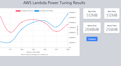
From this data a visualization is generated displaying execution times and average cost of the configuration. Neat. An example can be seen below:

Scenario

We’ll test this against a real Lambda service used over at Moonpig. From digging around in logs I observed a specific non I/O operation appeared quite slow and likely CPU bound, a great case for the power tuning tool!

Against 30 invocations per memory setting, the initial results we disappointing since increasing memory should yield something fairly linear, however, that’s not the case. After some digging a third-party service had varied response times for each call, therefore, skewing the results.

Since the goal of this is to determine optimal CPU usage and I/O operations are not a factor, all I/O calls were removed to create a more deterministic computation, allowing us to focus on the specific code computation mentioned above, Any HTTP calls were mocked.

Round 2

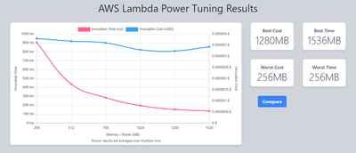
This produced the desired result, with a much more linear progression, costs remaining similar throughout each configuration due to consistent time reductions.

Since the higher value memory performed best, a macro-level approach was taken, starting from the best result of 1536MB in the previous test and incrementally scaling up to 3072MB. The x-axis shows all values used.

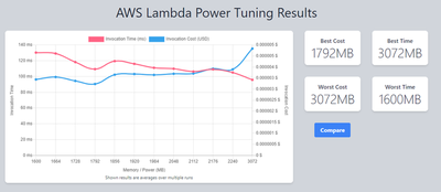
Depending on optimization preference on cost vs performance, we can see 1792MB being the lowest cost at 2240MB we save < 10ms but the additional cost isn’t worth it for a service that isn’t latency-sensitive in this case.

Conclusion

From our deterministic setup, we’ve improved from 900ms to less than 100ms whilst fractionally reducing cost.

This is a time reduction of 88.8% 🔥 for the computation without much work. Given how easy it is to do this, I would encourage you to give it a try.